
Time series forecasting with XGBoost and InfluxDB
XGBoost is an open source machine learning library that implements optimized distributed gradient boosting algorithms. XGBoost uses parallel processing for fast performance, handles missing values well, performs well on small datasets, and prevents overfitting. All of these advantages make XGBoost a popular solution for regression problems such as forecasting.
Forecasting is a critical task for all kinds of business objectives, such as predictive analytics, predictive maintenance, product planning, budgeting, etc. Many forecasting or prediction problems involve time series data. That makes XGBoost an excellent companion for InfluxDB, the open source time series database.
In this tutorial we’ll learn about how to use the Python package for XGBoost to forecast data from InfluxDB time series database. We’ll also use the InfluxDB Python client library to query data from InfluxDB and convert the data to a Pandas DataFrame to make working with the time series data easier. Then we’ll make our forecast.
I’ll also dive into the advantages of XGBoost in more detail.
Requirements
This tutorial was executed on a macOS system with Python 3 installed via Homebrew. I recommend setting up additional tooling like virtualenv, pyenv, or conda-env to simplify Python and client installations. Otherwise, the full requirements are these:
- influxdb-client = 1.30.0
- pandas = 1.4.3
- xgboost >= 1.7.3
- influxdb-client >= 1.30.0
- pandas >= 1.4.3
- matplotlib >= 3.5.2
- sklearn >= 1.1.1
This tutorial also assumes that you have a free tier InfluxDB cloud account and that you have created a bucket and created a token. You can think of a bucket as a database or the highest hierarchical level of data organization within InfluxDB. For this tutorial we’ll create a bucket called NOAA.
Decision trees, random forests, and gradient boosting
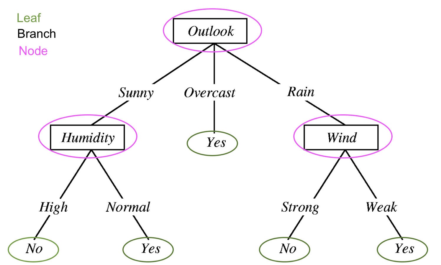
In order to understand what XGBoost is, we must understand decision trees, random forests, and gradient boosting. A decision tree is a type of supervised learning method that’s composed of a series of tests on a feature. Each node is a test and all of the nodes are organized in a flowchart structure. The branches represent conditions that ultimately determine which leaf or class label will be assigned to the input data.
 Prince Yadav
A decision tree for determining whether it will rain from Decision Tree in Machine Learning. Edited to show the components of the decision tree: leaves, branches, and nodes.
The guiding principle behind decision trees, random forests, and gradient boosting is that a group of “weak learners” or classifiers collectively make strong predictions.
A random forest contains several decision trees. Where each node in a decision tree would be considered a weak learner, each decision tree in the forest is considered one of many weak learners in a random forest model. Typically all of the data is randomly divided into subsets and passed through different decision trees.
Gradient boosting using decision trees and random forests are similar, but they differ in the way they’re structured. Gradient-boosted trees also contain a forest of decision trees, but these trees are built additively and all of the data passes through a collection of decision trees. (More on this in the next section.) Gradient-boosted trees may contain a set of classification or regression trees. Classification trees are used for discrete values (e.g. cat or dog). Regression trees are used for continuous values (e.g. 0 to 100).
What is XGBoost?
Gradient boosting is a machine learning algorithm that is used for classification and predictions. XGBoost is just an extreme type of gradient boosting. It’s extreme in the way that it can perform gradient boosting more efficiently with the capacity for parallel processing. The diagram below from the XGBoost documentation illustrates how gradient boosting might be used to predict whether an individual will like a video game.
 xgboost developers
Two trees are used to decide whether or not an individual will be likely to enjoy a video game. The leaf score from both trees is added to determine which individual will be most likely to enjoy the video game.
See Introduction to Boosted Trees in the XGBoost documentation to learn more about how gradient-boosted trees and XGBoost work.
Some advantages of XGBoost:
- Relatively easy to understand.
- Works well on small, structured, and regular data with few features.
Some disadvantages of XGBoost:
- Prone to overfitting and sensitive to outliers. It might be a good idea to use a materialized view of your time series data for forecasting with XGBoost.
- Doesn’t perform well on sparse or unsupervised data.
Time series forecasts with XGBoost
We’re using the Air Sensor sample dataset that comes out of the box with InfluxDB. This dataset contains temperature data from multiple sensors. We’re creating a temperature forecast for a single sensor. The data looks like this:
 InfluxData
Use the following Flux code to import the dataset and filter for the single time series. (Flux is InfluxDB’s query language.)
import "join"
import "influxdata/influxdb/sample"
//dataset is regular time series at 10 second intervals
data = sample.data(set: "airSensor")
  |> filter(fn: (r) => r._field == "temperature" and r.sensor_id == "TLM0100")
Random forests and gradient boosting can be used for time series forecasting, but they require that the data be transformed for supervised learning. This means we must shift our data forward in a sliding window approach or lag method to convert the time series data to a supervised learning set. We can prepare the data with Flux as well. Ideally you should perform some autocorrelation analysis first to determine the optimal lag to use. For brevity, we will just shift the data by one regular time interval with the following Flux code.
import "join"
import "influxdata/influxdb/sample"
data = sample.data(set: "airSensor")
  |> filter(fn: (r) => r._field == "temperature" and r.sensor_id == "TLM0100")
shiftedData = data
  |> timeShift(duration: 10s , columns: ["_time"] )
join.time(left: data, right: shiftedData, as: (l, r) => (l with data: l._value, shiftedData: r._value))
  |> drop(columns: ["_measurement", "_time", "_value", "sensor_id", "_field"])
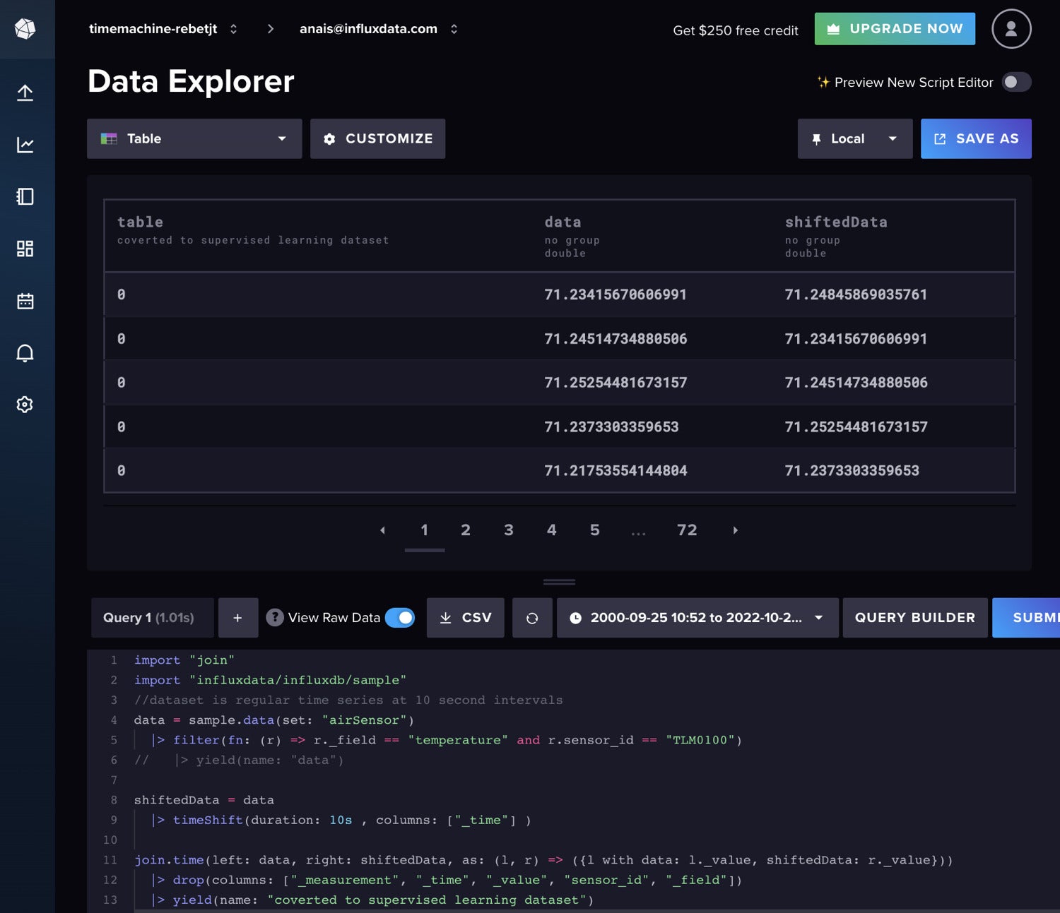 InfluxData
If you wanted to add additional lagged data to your model input, you could follow the following Flux logic instead.
import "experimental"
import "influxdata/influxdb/sample"
data = sample.data(set: "airSensor")
|> filter(fn: (r) => r._field == "temperature" and r.sensor_id == "TLM0100")

shiftedData1 = data
|> timeShift(duration: 10s , columns: ["_time"] )
|> set(key: "shift" , value: "1" )

shiftedData2 = data
|> timeShift(duration: 20s , columns: ["_time"] )
|> set(key: "shift" , value: "2" )

shiftedData3 = data
|> timeShift(duration: 30s , columns: ["_time"] )
|> set(key: "shift" , value: "3")

shiftedData4 = data
|> timeShift(duration: 40s , columns: ["_time"] )
|> set(key: "shift" , value: "4")

union(tables: [shiftedData1, shiftedData2, shiftedData3, shiftedData4])
|> pivot(rowKey:["_time"], columnKey: ["shift"], valueColumn: "_value")
|> drop(columns: ["_measurement", "_time", "_value", "sensor_id", "_field"])
// remove the NaN values
|> limit(n:360)
|> tail(n: 356)
In addition, we must use walk-forward validation to train our algorithm. This involves splitting the dataset into a test set and a training set. Then we train the XGBoost model with XGBRegressor and make a prediction with the fit method. Finally, we use MAE (mean absolute error) to determine the accuracy of our predictions. For a lag of 10 seconds, a MAE of 0.035 is calculated. We can interpret this as meaning that 96.5% of our predictions are very good. The graph below demonstrates our predicted results from the XGBoost against our expected values from the train/test split.
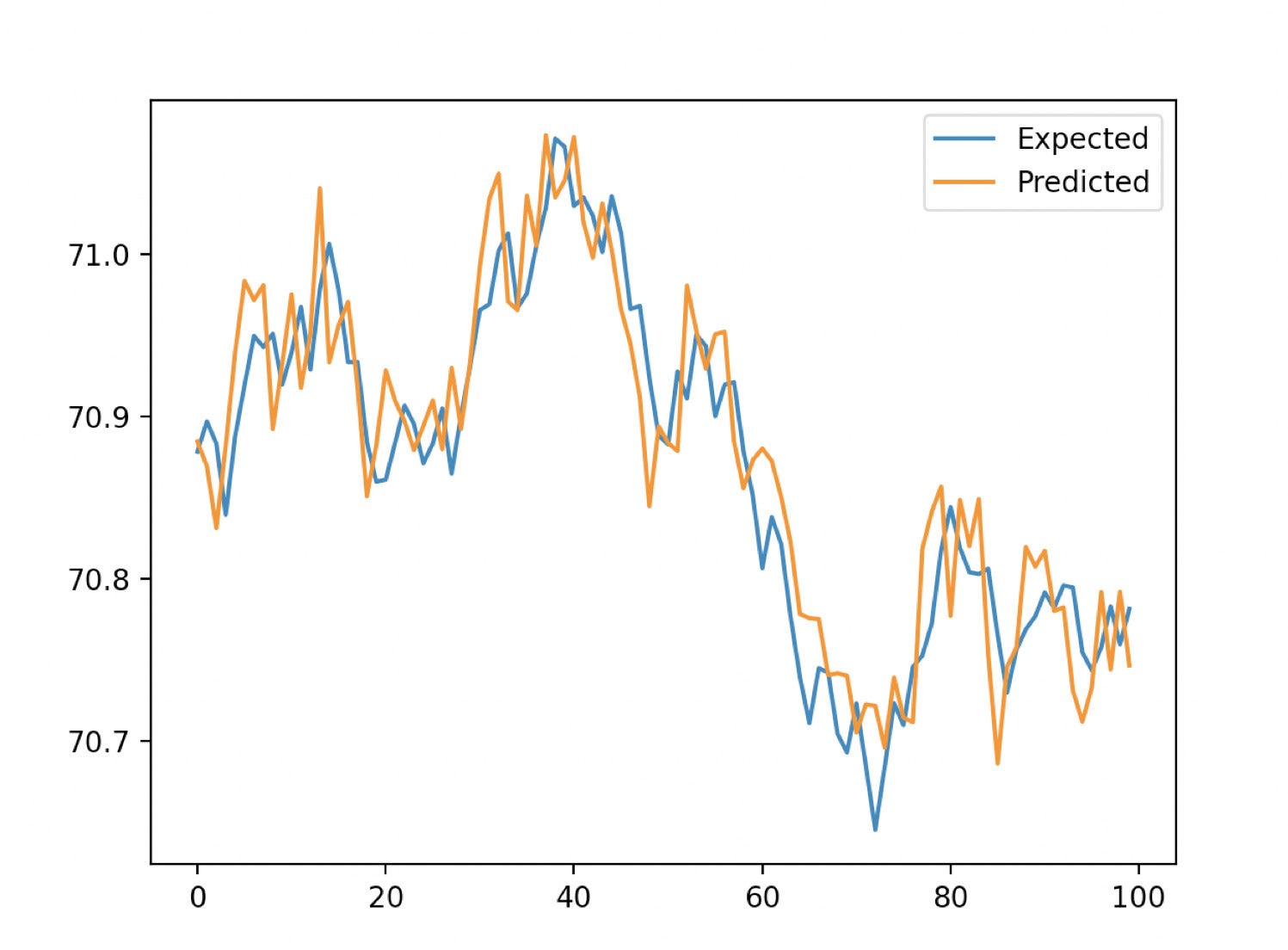 InfluxData
Below is the full script. This code was largely borrowed from the tutorial here.
import pandas as pd
from numpy import asarray
from sklearn.metrics import mean_absolute_error
from xgboost import XGBRegressor
from matplotlib import pyplot
from influxdb_client import InfluxDBClient
from influxdb_client.client.write_api import SYNCHRONOUS

# query data with the Python InfluxDB Client Library and transform data into a supervised learning problem with Flux
client = InfluxDBClient(url="https://us-west-2-1.aws.cloud2.influxdata.com", token="NyP-HzFGkObUBI4Wwg6Rbd-_SdrTMtZzbFK921VkMQWp3bv_e9BhpBi6fCBr_0-6i0ev32_XWZcmkDPsearTWA==", org="0437f6d51b579000")

# write_api = client.write_api(write_options=SYNCHRONOUS)
query_api = client.query_api()
df = query_api.query_data_frame('import "join"'
'import "influxdata/influxdb/sample"'
'data = sample.data(set: "airSensor")'
  '|> filter(fn: (r) => r._field == "temperature" and r.sensor_id == "TLM0100")'
'shiftedData = data'
  '|> timeShift(duration: 10s , columns: ["_time"] )'
'join.time(left: data, right: shiftedData, as: (l, r) => (l with data: l._value, shiftedData: r._value))'
  '|> drop(columns: ["_measurement", "_time", "_value", "sensor_id", "_field"])'
  '|> yield(name: "converted to supervised learning dataset")'
)
df = df.drop(columns=['table', 'result'])
data = df.to_numpy()

# split a univariate dataset into train/test sets
def train_test_split(data, n_test):
     return data[:-n_test:], data[-n_test:]

# fit an xgboost model and make a one step prediction
def xgboost_forecast(train, testX):
     # transform list into array
     train = asarray(train)
     # split into input and output columns
     trainX, trainy = train[:, :-1], train[:, -1]
     # fit model
     model = XGBRegressor(objective="reg:squarederror", n_estimators=1000)
     model.fit(trainX, trainy)
     # make a one-step prediction
     yhat = model.predict(asarray([testX]))
     return yhat[0]

# walk-forward validation for univariate data
def walk_forward_validation(data, n_test):
     predictions = list()
     # split dataset
     train, test = train_test_split(data, n_test)
     history = [x for x in train]
     # step over each time-step in the test set
     for i in range(len(test)):
          # split test row into input and output columns
          testX, testy = test[i, :-1], test[i, -1]
          # fit model on history and make a prediction
          yhat = xgboost_forecast(history, testX)
          # store forecast in list of predictions
          predictions.append(yhat)
          # add actual observation to history for the next loop
          history.append(test[i])
          # summarize progress
          print('>expected=%.1f, predicted=%.1f' % (testy, yhat))
     # estimate prediction error
     error = mean_absolute_error(test[:, -1], predictions)
     return error, test[:, -1], predictions

# evaluate
mae, y, yhat = walk_forward_validation(data, 100)
print('MAE: %.3f' % mae)

# plot expected vs predicted
pyplot.plot(y, label="Expected")
pyplot.plot(yhat, label="Predicted")
pyplot.legend()
pyplot.show()
Conclusion
I hope this blog post inspires you to take advantage of XGBoost and InfluxDB to make forecasts. I encourage you to take a look at the following repo which includes examples for how to work with many of the algorithms described here and InfluxDB to make forecasts and perform anomaly detection.
Anais Dotis-Georgiou is a developer advocate for InfluxData with a passion for making data beautiful with the use of data analytics, AI, and machine learning. She applies a mix of research, exploration, and engineering to translate the data she collects into something useful, valuable, and beautiful. When she is not behind a screen, you can find her outside drawing, stretching, boarding, or chasing after a soccer ball.
—
New Tech Forum provides a venue to explore and discuss emerging enterprise technology in unprecedented depth and breadth. The selection is subjective, based on our pick of the technologies we believe to be important and of greatest interest to InfoWorld readers. InfoWorld does not accept marketing collateral for publication and reserves the right to edit all contributed content. Send all inquiries to [email protected].
Copyright © 2022 IDG Communications, Inc.


